Machine Learning and Statistical Analysis
title: Machine Learning and Statistical Analysis description: London Bike Sharing demand prediction in R date: 2024-01-23
Machine Learning and Statistical Analysis
London Bike Sharing demand prediction in R

Introduction
The London Bike Sharing Dataset provides a detailed view of bike rental demand across hourly time intervals, enriched with weather and calendar information. In this project, I use R to explore the dataset, engineer time-based features, and train multiple regression models to predict hourly bike rental demand (cnt). The workflow includes data cleaning, exploratory analysis, outlier handling, model training, and performance comparison.
Project Objectives
- Data preprocessing: clean data, handle missing values, and align variable types.
- Exploratory data analysis (EDA): identify trends, seasonality, and relationships with weather/time features.
- Feature engineering: extract
year,month,day, andhourfrom the timestamp and prepare categorical features. - Model development: train and compare multiple regression models in R.
- Evaluation: assess models using RMSE, MSE, and R-squared (with and without outliers).
- Insights: highlight key drivers of bike demand and practical takeaways.
Data Source
- Dataset: London Bike Sharing Dataset (Kaggle)
https://www.kaggle.com/datasets/hmavrodiev/london-bike-sharing-dataset
Core features used:
timestamp: observation time (used for feature extraction)cnt: total hourly rentals (target)t1,t2: temperature and “feels like” temperaturehum: humiditywind_speed: wind speedweather_code: weather condition categoryis_holiday,is_weekend: calendar flagsseason: meteorological season category
Tools and Technologies
- R / RStudio
- Key packages:
dplyr,tibble,lubridate(wrangling + time features)ggplot2,scales,gridExtra(visualization)caret(splits, preprocessing)rpart,randomForest,xgboost(modeling)skimr,PerformanceAnalytics(profiling & correlation)
Methodology
1) Data Loading and Feature Engineering
After loading the dataset, I extracted time features (year, month, day, hour) from timestamp, then removed the original timestamp from modeling features.
2) Data Quality Checks
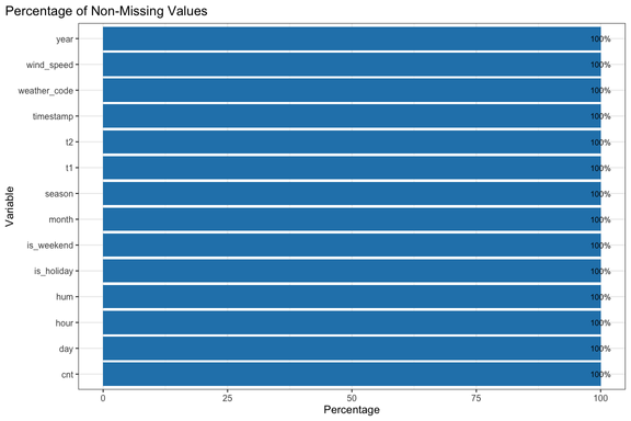
I inspected missing values, verified variable types, and reviewed summary statistics before modeling.
3) Exploratory Data Analysis
EDA focused on:
- distribution of bike rentals (
cnt) and outliers - relationships with
t1,hum, andwind_speed - seasonality by month and hour (rush-hour patterns)
- categorical impacts (holiday/weekend/weather/season)

4) Feature Selection Notes
Two important adjustments were made for more reliable modeling:
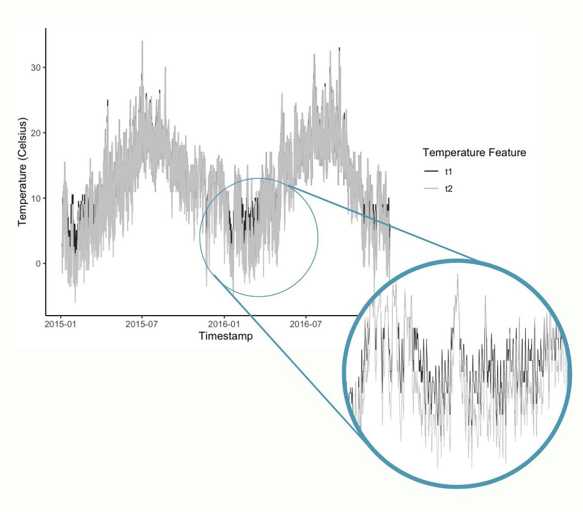
- Dropped
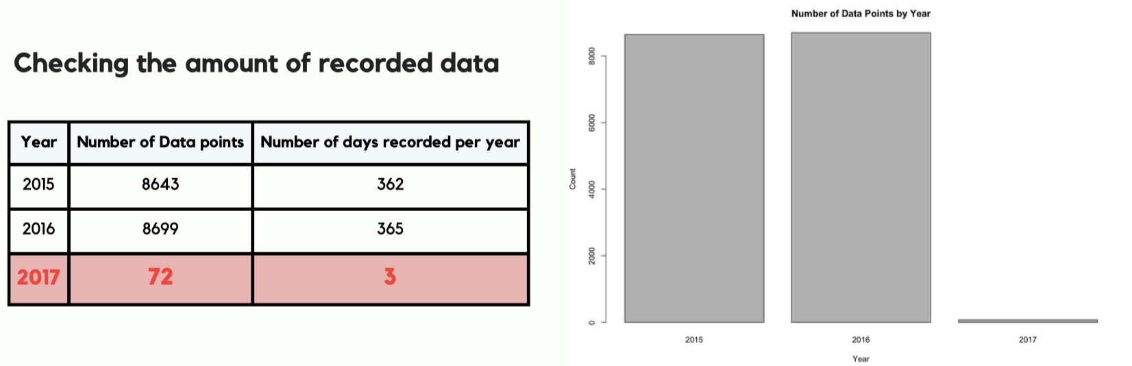
t2after confirming it was highly correlated witht1but less reliable for consistency. - Excluded year 2017 due to significantly fewer observations than 2015–2016 (avoids imbalance and improves generalization).
Modeling and Evaluation
Train/Test Split + Scaling
The dataset was split into training and testing subsets (80/20). Numeric features were standardized where required, then recombined with categorical variables.
Models Compared
- Linear Regression (baseline)
- Decision Tree (
rpart) - XGBoost (
xgboost) - Random Forest (
randomForest)
Metrics
- MSE (Mean Squared Error)
- RMSE (Root Mean Squared Error)
- R-squared (explained variance)
Model performance was compared with and without outliers to evaluate sensitivity to extreme demand spikes.
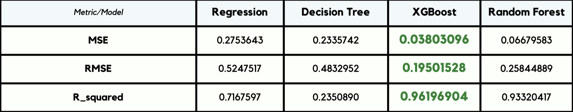
Key Results
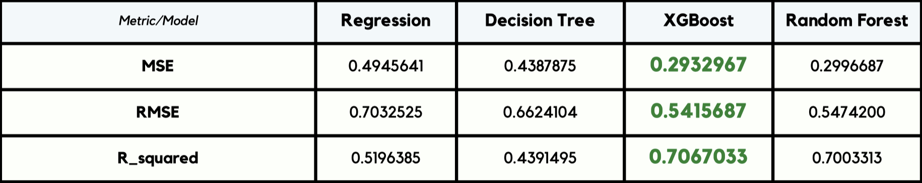
- XGBoost delivered the strongest overall performance (lowest error, highest R²).
- Random Forest was consistently competitive and robust.
- Removing outliers improved all models, especially the ensemble methods.
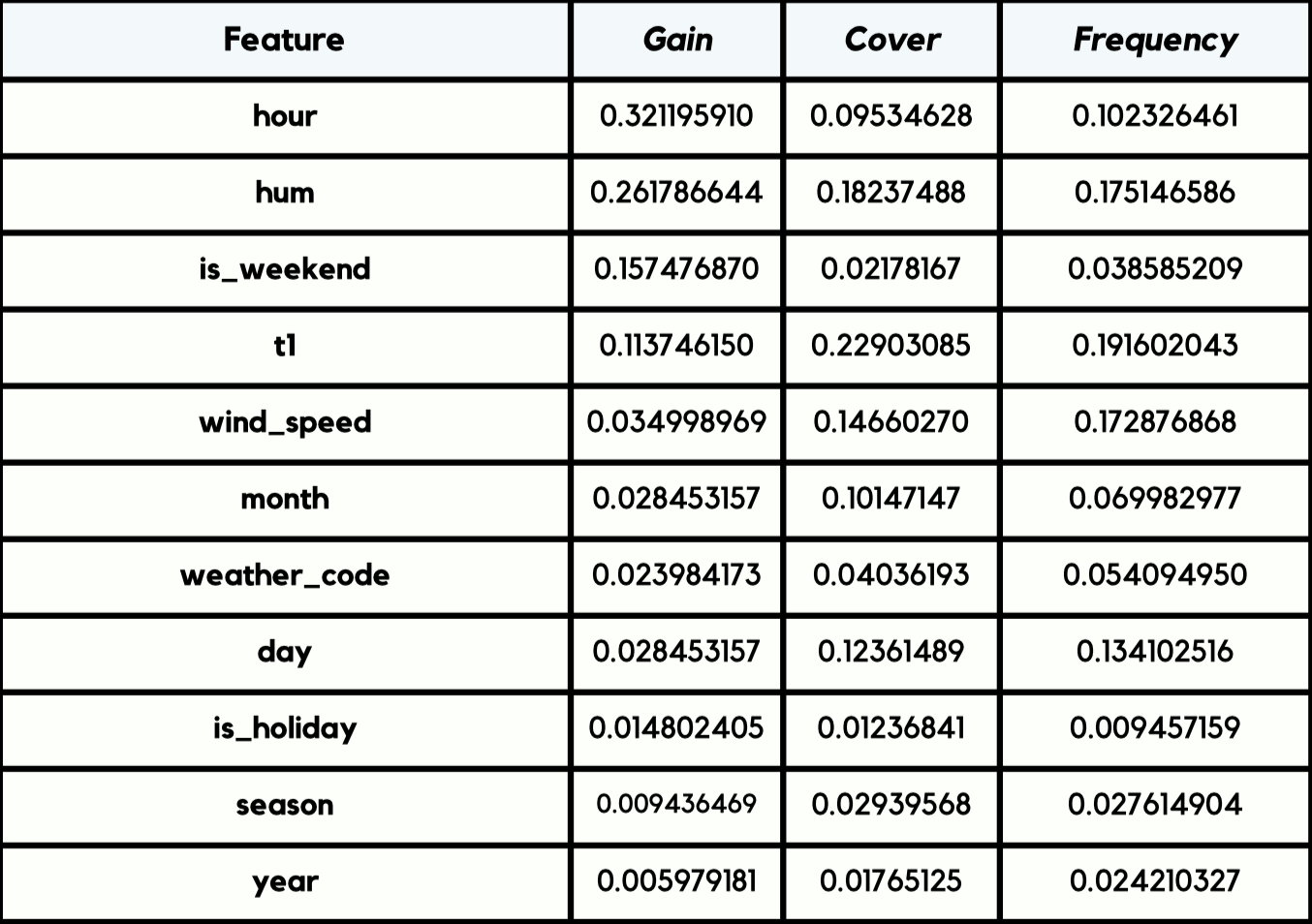
Insights
From both EDA and model behavior, the strongest demand drivers were:
- Time of day (commute peaks in the morning and late afternoon)
- Temperature
- Humidity
- Season / weather condition
These signals are useful for operational planning—bike redistribution, staffing, and expected demand forecasting.
Conclusion
This project demonstrates an end-to-end machine learning workflow in R, applied to a real-world urban mobility dataset. By combining statistical thinking, careful preprocessing, and model benchmarking, I built predictive models capable of estimating hourly bike demand in London. Ensemble methods—especially XGBoost—performed best, and outlier handling proved essential for improving accuracy.
Source Code and Resources
-
London Bike Sharing dataset (
.csv):
https://github.com/pouyasattari/Statistical-Data-Analysis-London-Bike-Sharing-Dataset/blob/main/london_merged.csv -
Main project code (
.Rmd) + PDF export:
https://github.com/pouyasattari/Statistical-Data-Analysis-London-Bike-Sharing-Dataset/blob/main/R%20markdown%20Project.Rmd
https://github.com/pouyasattari/Statistical-Data-Analysis-London-Bike-Sharing-Dataset/blob/main/Project-edited.pdf -
Technical report (
.pdf):
https://github.com/pouyasattari/Statistical-Data-Analysis-London-Bike-Sharing-Dataset/blob/main/%20Technical%20Report.pdf -
Presentation (
.pdf):
https://github.com/pouyasattari/Statistical-Data-Analysis-London-Bike-Sharing-Dataset/blob/main/London%20Bike%20Sharing_Presentation.pdf -
GitHub repository:
https://github.com/pouyasattari/London-Bike-Sharing-Statistical-Data-Analysis-in-R